

Ronan Armstrong
Musician, educator, developer, author, and all-around nerd. From producing genre-bending alternative pop and rock to tracking the sound effects for independent game studios, I bring unparalleled expertise and insight to any project.
Recording
As an engineer, I’ve worked with countless artists across a multitude of genres. My deep technical knowledge and creative insight can help your musical ideas come to life.
Composition
With more then 20 composition and arrangement awards, I can take your melody or lyrics to a full contemporary production.
Development
Whether you’re developing audio plugins, deeply integrated intranet systems, or something as simple as a portfolio website, I work with my clients to deliver powerful, performant designs.
Recent Projects
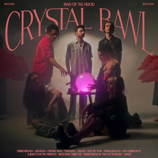
Crystal Bawl
Executive Producer, Engineer, Programming, Viola
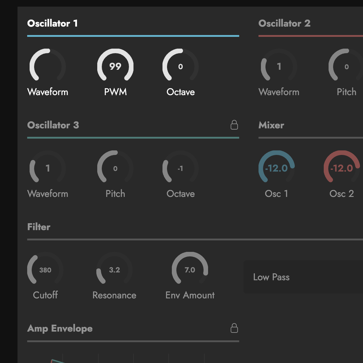
MasterELM
Development, UI, Synthesis Consultant, Preset Designer
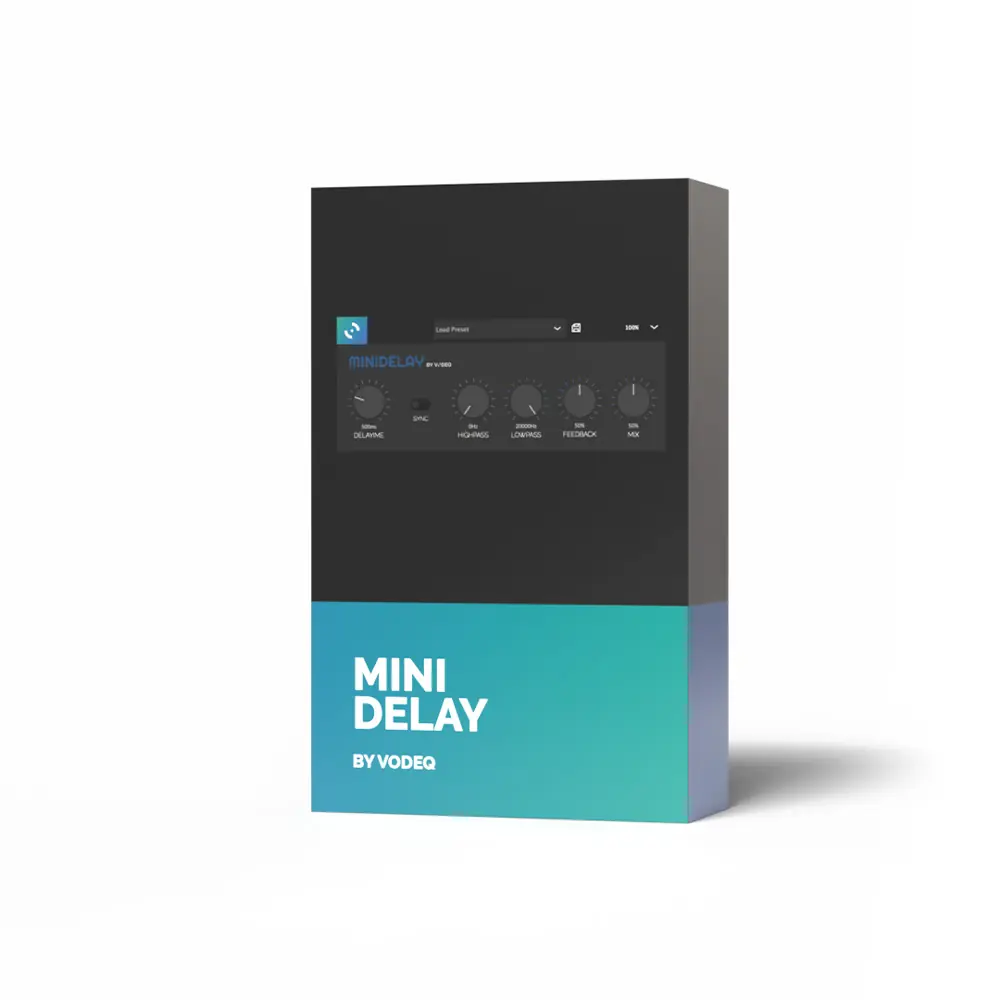
MiniDelay
Senior DSP Developer, Product Design Specialist
About Me
I’ve spent my entire life studying music, from classical composition and arrangement to technical recording. With over fifteen years of experience in contemporary music production, a handful of degrees from the best production colleges in the world, and an undying love for anything vintage, I’m the perfect choice for your next project.


“Ronan can speak to an uncanny breadth of subjects with unprecedented depth. As a colleague I’ve found him to be a renaissance man of all things audio, from technical design to artistic implementation. He’s a good hang, too.”
Ryan Tilby, Producer & Mix Engineer